Imagery
ESD gliders may be equipped with either a ‘glidercam’ or a ‘shadowgraph’ camera. This page describes the management and processing of these images once they come off of the glider.
Raw Imagery
Once the gliders are recovered, the glidercam or shadowgraph directories and images are copied from the memory cards and uploaded to GCP as described in Data Management. Specifically, raw images and config files are uploaded to the raw imagery bucket. Image metadata files generated during the base glider data processing are written to the deployment’s ‘metadata’ folder within this bucket (see below for more details).
Imagery metadata
Viewing Images
There are several ways to view raw or processed images:
If you click down to an image itself, Google Cloud provides an image preview at the bottom of the ‘object’ page. However, you cannot view more than one image at a time. It is a goal of the ESD to build a cloud-native image viewer application to easily view multiple images at a time, but this is not a current project.
All raw imagery have been mirrored in VIAME-Web-AMLR. Thus, if you are familiar with VIAME-Web and accessing ESD’s deployment, then you can view imagery using the VIAME-Web annotator.
You may also use the gcloud CLI to download images to your computer, and then view them locally using your preferred program.
Shadowgraph Image Processing
NOTE: Given personnel changes, this section is out of date. Contact Jen Walsh or Sam Woodman for latest image processing efforts, in particular through the Optics SI
Gliders deployed with shadowgraph cameras can easily collect more than 200,000 images during a single deployment. Therefore, it is impractical to have humans review and annotate all these images by hand, and thus operationally these images must be processed using AI/ML methods. This section describes the current status of these methods, as well as anticipated future directions.
There are three main steps to processing shadowgraph images; where and how these steps happen for ESD are further described below.
- Preprocessing: flat-fielding, masking, other processing as needed.
- Segmentation: Detect objects, and create regions of interest (ROIs; i.e., blobs or chips). This is done using the preprocessed image.
- Classification: Use a trained ML model to classify the ROIs. Have a trained biologist review and/or correct these predictions.
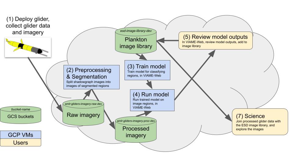
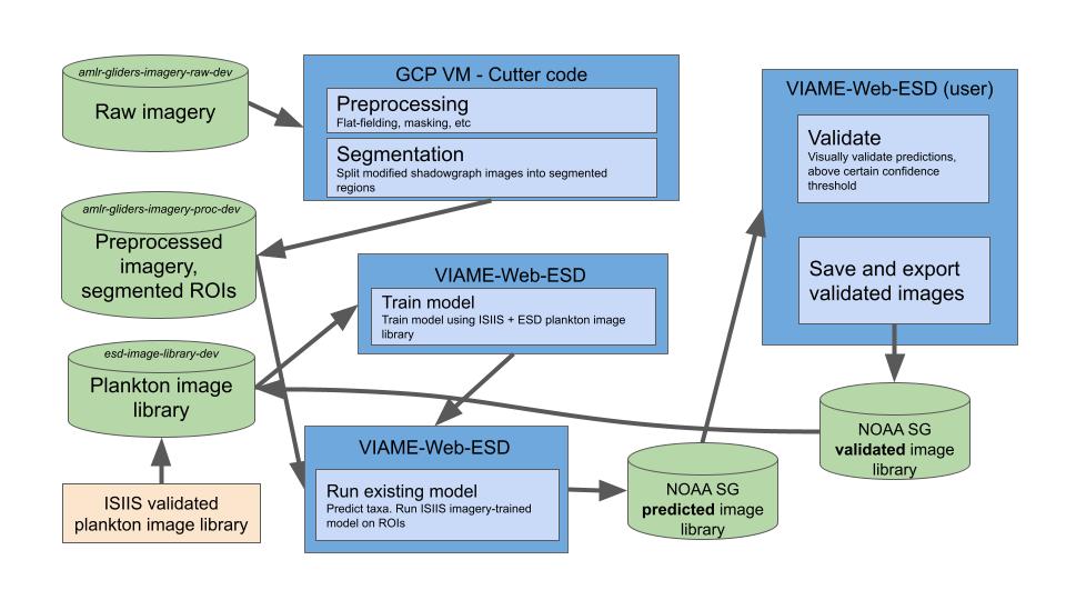
Note: the below images both show this same workflow, and thus are simply different ways of framing said workflow.
 Shadowgraph image processing workflow, v1
 Shadowgraph image processing workflow, v2
Preprocessing and Segmentation
All preprocessing and object detection/segmentation steps are currently performed by code in the shaip repo (shadowgraph image processing). This codebase was originally developed as a Jupyter notebook by Randy Cutter based on work done by Ohman/Ellen for processing Zooglider images, e.g. here and here. It has since been refactored into the Python toolbox sg. For details on the algorithms used and instructions on how to run this code, see the README on the repo homepage.
All currently processed imagery can be found in amlr-gliders-imagery-proc-dev. Like the raw imagery bucket, the amlr-gliders-imagery-proc-dev bucket mirrors the directory structure of the amlr-gliders-deployments-dev bucket. These processed imagery are also viewable as described above.
The processing output includes the following folders:
- regions: Region of interest (ROI) blobs, created using Ohman/Ellen methods. This folder contains Dir#### folders, matching the raw data.
- regions-tmser: Region of interest (ROI) blobs, created using an adapted version of Oregon State’s Threshold MSER In Situ Plankton Segmentation. Most deployments do not have this output, as this method has not been tuned to work well with ESD shadowgraph imagery.
- jpgorig-regions: jpg of the original (i.e., raw) image, with ROI boundaries from the Ohman/Ellen segmentation methods outlined in red.
- images-imgff: Flat-fielded images, used in the segmentation
- images-ffPCG: Flat-fielded images, which also have had pixel gamma correction factors applied.
Classification
After creating ROIs through the preprocessing and segmentation steps described above, those ROIs need to be labeled/classified, and these labels/classifications need to be validated by a trained observer.
Model Training
To train an ML model to classify the ROIs as different classes, e.g. plankton species requires an image library of already-classified images that can be used as ground-truth data for the model. ESD is currently using the In Situ Ichthyoplankton Imaging System (ISIIS) image library, courtesy of researchers at Oregon State University, for training full frame classifier models. This library consists of 174 classes of objects, and can be found here.
In early 2024, Randy used the ISIIS image library to train two models using VIAME-Web-AMLR (VWA): isiis-train02-clas-svm-lab81, and isiis-train02-clas-res01-lab81. Both of these models have 81 classes, and are available in VWA. Per Randy, the resnet (isiis-train02-clas-res01-lab81) theoretically should be better, but has so far been outperformed by the SVM. This is probably because of not enough training data relative to the number of input classes. Randy also was experimenting with training a yolo v7 model, but this model was not really tested. Thus, currently the resnet is the best model that we have for running on segmented ROIs.
Generating and Validating Predictions
NOTE: these steps of running a model on ROIs and validating subsequent predictions are currently on hold. Specifically, ESD is currently pushing down two paths in parallel: 1) evaluating and improving current preprocessing and segmentation efforts, and 2) performing manual annotations on raw imagery, and extracting user-annotated ROIs to build an ESD image library.
For information on how to run these models on a folder of ROIs, see here. For information about how to validate model predictions, see here.
Future Directions
Tune and adapt current code/pipelines (in progress). This work is currently being done by ESD staff.
Work to tune and evaluate alternative segmentation algorithms, e.g. https://github.com/paradom/Threshold-MSER
Tie in with Optics SI efforts, e.g. https://github.com/sullichrosu/Njobvu-AI
